Data processing in AI, ML is a crucial step. Collected raw data is often messy and inconsistent. In this step, it is transformed into usable data for AI/ML algorithms. This allows them to learn and produce desirable results. It’s the foundation upon which accurate and reliable models are built. Simply, raw data needs to processed to make it useful for AI/ML.

Why data processing is crucial?

• Raw data is often messy and inconsistent. It often has missing values, outliers, noise and errors.
• AI/ML models depend upon quality of data per desirable result and performance.
• Unprocessed data can be large and complex. By cleansing, transforming and reducing dimensions, we make it easier for AI system to process.
• By removing unnecessary features, noise and outliers over-fitting can be prevented to the training data.
• Different AI/ML algorithms required different format of data for processing.

Preprocessing Steps

Data collection, cleansing, integration, transformation, feature engineering, splitting and balancing are the crucial steps in preprocessing. Today, I learned about how to handle missing values and feature scaling.

Handling Missing Values

One simple way to handle missing values is to remove the entire row or column of data. However, this method may result in significant data loss.

Another method is to use mean, median or mode of that column for the missing value. It may result distortion in the relationship among variable or reduce variance.

Feature Scaling

Feature scaling normalize or standardize numerical features to ensure fair influence on the model. This is important for learning algorithms sensitive to magnitude and range of input features.

Today I learned StandardScaler from scikit-learn python library. But it also provide other scaling mechanism e.g. MinMaxScaler, RobustScaler, MaxAbsScaler, Normalizer etc.

StandardScaler

StandardScaler transforms data into feature such that mean is 0 and standard deviation is 1. The formula for standardization of a given feature x is

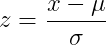
where:

• x is the original value of the feature.
• mu (μ) is the mean of the feature in the training data.
• sigma (σ) is the standard deviation of the feature in the training data.

Coding

import pandas as pd
from sklearn.preprocessing import StandardScaler

# Load Iris dataset
df = pd.read_csv('https://raw.githubusercontent.com/mwaskom/seaborn-data/master/iris.csv')
print("Dataset Head:\n", df.head())

# Check for missing values
print("Missing Values:\n", df.isnull().sum())

# Handle missing values (fill with mean for numerical columns)
df.fillna(df.mean(numeric_only=True), inplace=True)

# Scale numerical features (exclude 'species' column)
scaler = StandardScaler()
X = df.drop('species', axis=1)  # Features
X_scaled = scaler.fit_transform(X)
print("Scaled Features (first 5 rows):\n", X_scaled[:5])

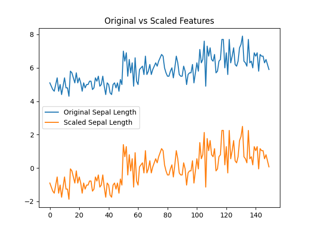
Original vs. Scaled Data

import matplotlib.pyplot as plt
plt.plot(df['sepal_length'], label='Original Sepal Length')
plt.plot(X_scaled[:, 0], label='Scaled Sepal Length')
plt.legend()
plt.title('Original vs Scaled Features')
plt.savefig('my_plot.png')
plt.show()

Output Graph