Linear Regression
Linear regression is a statistical method. It is used to model relationship between a dependent variable and one or more independent variable. The primary objective of linear regression is to predict the dependent variable’s value. This prediction is based on the values of the independent variables.
Here are key aspects of Linear Regression:
Simple Linear Regression
This involves two variables – one dependent and one independent variable. The relationship is modeled using linear equation
y = β0 + β1x + ε
where
- y is the dependent variable.
- x is the independent variable.
- β0 is the intercept.
- β1 is the slope.
- ε is the error term.
Example: Predicting sepal_width from sepal_length in iris dataset.
Multiple Linear Regression
This extends simple linear regression by incorporating multiple independent variables. The equation is:
y = β0 + β1x1 + β2x2 + … + βnxn + ε
where x1, x2, …, xn are independent variables.
Example: Predicting sepal_width from sepal_length, petal_length, petal_width in iris dataset.
Linear regression assumes a linear relationship between the dependent and independent variables, homoscedasticity (constant variance of error), independence of observations and normally distributed errors.
Linear Regression is widely used in various fields like finance, biology, and economics to predict the outcomes and analyze relationship between variables.
Homoscedasticity
Homoscedasticity refers to the assumption that the variance of errors (residuals) is constant across all levels of the independent variable(s). In simpler terms, it means that the spread or dispersion of the errors should be roughly the same. In linear regression, residuals are the differences between the observed values of the dependent variable and the predicted values by the regression model. This holds true regardless of the value of the independent variable. This assumption is crucial for the validity of statistical inference drawn from the regression model. Violation of it can lead to biased estimates and unreliable predictions.
Variance
Variance measures the dispersion or spread of data points around their mean. It quantifies how much data points deviate from the average value. Formula for variance is:
s2 = (1 / (n − 1)) Σ(xi − x̄)2
Where
- s2 is sample variance.
- n is sample size.
- xi is i-th data point.
- x̄ is mean of the dataset.
Example Calculation
Let say we have a sample of exam score: 85, 90, 78, 92 and 88.
| Index | xi (score) | xi − x̄ (deviation) | (xi − x̄)2 (squared deviation) |
|---|---|---|---|
| 1 | 85 | -1.6 | 2.56 |
| 2 | 90 | 3.4 | 11.56 |
| 3 | 78 | -8.6 | 73.96 |
| 4 | 92 | 5.4 | 29.16 |
| 5 | 88 | 1.4 | 1.96 |
| Total | 0 | 119.20 | |
| Mean (x̄) | 86.6 | ||
| Sample Variance (s2) | 29.8 |

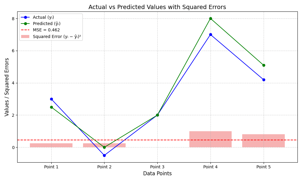
Mean Squared Error
Mean Squared Error (MSE) is a measure of the average squared difference between predicted and actual values in the dataset. It’s a common metrics used to evaluate the performance of regression models. A lower MSE indicates a better fir of the model to the data, as it signifies smaller average errors. Formula for Mean Squared Error:
MSE = (1 / n) Σ(yi − ŷi)2
Where
- MSE is Mean Squared Error.
- n is sample size.
- yi actual value of the data point.
- ŷi predicted value of the data point.
Example Calculation
| Index | Actual (yi) | Predicted (ŷi) | Error (yi – ŷi) | Squared Error (yi − ŷi)2 |
|---|---|---|---|---|
| 1 | 3.0 | 2.5 | 0.5 | 0.250 |
| 2 | -0.5 | 0.0 | -0.5 | 0.250 |
| 3 | 2.0 | 2.0 | 0.0 | 0.000 |
| 4 | 7.0 | 8.0 | -1.0 | 1.000 |
| 5 | 4.2 | 5.1 | -0.9 | 0.810 |
| Total: 2.360 | ||||
| MSE = 0.462 |
Coding
Training and comparing simple and multiple linear regression models to predict sepal_width in the Iris dataset. Evaluate with MSE. Visualize the regression results.
import pandas as pd
import matplotlib.pyplot as plt
from sklearn.model_selection import train_test_split
from sklearn.linear_model import LinearRegression
from sklearn.metrics import mean_squared_error

# Load Iris dataset
df = pd.read_csv('https://raw.githubusercontent.com/mwaskom/seaborn-data/master/iris.csv')

# Prepare data
X_Simple = df[['sepal_length']].values  # Simple: one feature
X_Multiple = df[['sepal_length', 'petal_length', 'petal_width']].values  # Multiple: three features
y = df['sepal_width'].values  # Target

# Split data (80% train, 20% test)
X_Simple_train, X_Simple_test, y_simple_train, y_simple_test = train_test_split(X_Simple, y, test_size=0.2, random_state=42)
X_Multiple_train, X_Multiple_test, y_multiple_train, y_multiple_test = train_test_split(X_Multiple, y, test_size=0.2, random_state=42)

# Simple Linear Regression
model_simple = LinearRegression()
model_simple.fit(X_Simple_train, y_simple_train)
y_simple_pred = model_simple.predict(X_Simple_test)
mse_simple = mean_squared_error(y_simple_test, y_simple_pred)
print("Simple Linear Regression MSE:", mse_simple)
print("Simple Coefficients:", model_simple.coef_, "Intercept:", model_simple.intercept_)

# Multiple Linear Regression
model_multiple = LinearRegression()
model_multiple.fit(X_Multiple_train, y_multiple_train)
y_multiple_pred = model_multiple.predict(X_Multiple_test)
mse_multiple = mean_squared_error(y_multiple_test, y_multiple_pred)
print("Multiple Linear Regression MSE:", mse_multiple)
print("Multiple Coefficients:", model_multiple.coef_, "Intercept:", model_multiple.intercept_)
Expected Output
Simple Linear Regression MSE: 0.13961895650579023
Simple Coefficients: [[-0.05829418]] Intercept: [3.40030729]
Multiple Linear Regression MSE: 0.08683537710785846
Multiple Coefficients: [[ 0.62934965 -0.63196673  0.6440201 ]] Intercept: [0.99870853]
Visualization
plt.figure(figsize=(10,6))
plt.scatter(X_Simple_test, y_simple_test, label='Actual')
plt.plot(X_Simple_test, y_simple_pred, color='red', label='Predicted')
plt.grid(True, linestyle='--', alpha=0.6)
plt.xlabel('Sepal Length')
plt.ylabel('Sepal Width')
plt.title('Simple Linear Regression')
plt.legend()
plt.tight_layout()
plt.show()


Leave a comment